Basics of multilabel classification

Multilabel dataset traits

The figure below outlines the measures. Some of the important measures have been explained below.

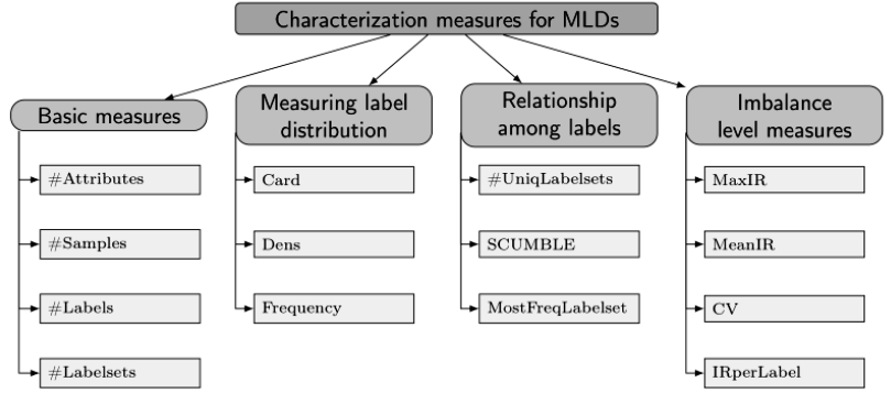
Basic measures :

The most basic information that can be obtained from an MLD is the number of instances, attributes and labels. Each instance has an associated labelset, whose length (number of active labels) can be in the range {0..|L|}.

Label related measures :

SCUMBLE (Score of ConcUrrence among iMBalanced LabEls): The joint presence of labels with different frequencies in the same instance can pose a challenge for resampling algorithms. It is used to assess the concurrence level among frequent and infrequent labels.

Card (Cardinality): The average number of active labels per instance.

Dens (Density): Dividing Card by the number of labels results in a dimension-less measure, known as Dens.

UniqLabelsets: The number of different labelsets and the amount of them being unique (appearing only once in sample). This gives us a glimpse on how sparsely the labels are distributed.

Imbalance related measures:

IRLb (Imbalance ratio per label): The level of imbalance of a determinate label can be measured by the imbalance ratio, known as IRLb. it is calculated for the label “l” as the ratio between the majority label and the label “l”. This value will be 1 for the most frequent label and a greater value for the rest. The larger the IRLbl is, the higher would be the imbalance level for the considered label.

Multilabel classification

There are two possibilities to deal with multi-label classification:
Algorithm adaptation:
Modify the existing algorithms taking into account the multilabel nature of the samples. For example- hosting more than one class in the leaves of a tree instead of only one.

Problem transformation:
Transforming the original data to make it suitable to existing traditional classification algorithms and combining the obtained predictions to build the labelsets given as output result. There are several transformation methods in literature. Three have been defined and used for our case study.

• Binary Relevance (BR):
  • It is an adaptation of OVA (one-vs-all) to the multilabel scenario and transforms the original multilabel dataset into several binary datasets.
  • Here an ensemble of binary classifiers is trained, one for each class. Each classifier predicts either the membership or the non-membership of one class. A union of all predicted classes is taken as the multi-label output.
  • The approach is popular because it is easy to implement, but ignores the possible correlations between class labels.
• Label Powerset (LP):
  • This method transforms the multilabel dataset into a multiclass dataset by using the labelset of each instance as class identifier.
  • This approach takes possible correlations between class labels into account unlike the BR.
  • The downside of the method is it has a high computational complexity and when the number of classes increases the number of distinct label combinations can grow exponentially.
• Classifier Chains (CC):
  • This method comprises a chain of binary classifiers \(C_0, C_1, . . . , C_m \) is constructed, where a classifier \(C_i\) uses the predictions of all the classifier \(C_j\) , where j < i.
  • The method takes into account label correlations.
  • The total number of classifiers needed for this approach is equal to the number of classes, but the training of the classifiers is more involved.

Evaluation metric

Evaluation measures for a multi-label classification problem needs discussion as it is different from multiclass/binary class problem. In single label classification the commonly used metrics are - accuracy, precision, recall, F1-measure, among others. In multi-label classification we cannot define misclassification as a hard correct or incorrect, but a prediction comprising subset of actual classes is deemed better than containg none of them.

Multilabel evaluation metrics are grouped into two main categories: example based and label based metrics.

• Example based metrics are computed individually for each instance, then averaged to obtain the final value.
• Label based metrics are computed per label, instead of per instance.

Some of the measures have been described below.

Hamming Loss (Example based)
Hamming Loss is is an example based measure. It is defined as the fraction of labels that are incorrectly predicted.

\(HL = \frac{1}{N . L} \sum_{l=1}^L\sum_{i=1}^N Y_{i,l} \oplus X_{i,l}\)

where denotes exlusive-or, \(X_{i,l} (Y_{i,l})\) stands for boolean that the i-th prediction contains the l-th label. For binary scenario (L=1) equals to (1 - accuracy).

Micro-average and Macro-average (Label based)
In order to measure the performance of a multi-class classifier we have to consider the average performance over all classes. There are two different ways of doing this called micro-averaging and macro-averaging.

Micro Average
In micro, all TPs, TNs, FPs and FNs for each class are summed up and then the average is taken. The micro-average F1 is the harmonic mean of the below two equations.

\(Microaverage Precision Prc^{micro}(D) = \frac{\sum_c TP_c}{\sum_c TP_c + \sum_c FP_c} \)

\(Microaverage Recall Rcl^{micro}(D) = = \frac{\sum_c TP_c}{\sum_c TP_c + \sum_c FN_c} \)

Macro Average
In macro average we take the average of precision and recall of the system on different sets. It is used when we want to know how the algorithm performs overall across different subset of data.

\(Macrooaverage Precision Prc^{macro}(D) = \frac{\sum_c Prc(D,c)}{|C|} \)

\(Microaverage Recall Rcl^{macro}(D) = \frac{\sum_c Rcl(D,c)}{|C|} \)

In a multi-class classification setup, micro-average is preferable if there is class imbalance.

Subset accuracy (Example based)
It is the most strict evaluation metric. It indicates the percentage of samples that have all their labels classified correctly. The downside of this measure is that it is too strcit to be true, i.e - it ignores the partially correct matches. In a dataset having huge number of labels it is very challenging to get a good score for this measure.