Classification
The EUR-Lex dataset contains 25K documents, which makes it impossible to train a classifier over the whole dataset. We have divided the dataset into 25 subsets, therefore each subset contains 1000 documents. We trained the classifiers over the subsets. The final evaluations results will be the average over the subsets.
Classification Models
We have used three multilabel transformation methods : Binary relevance (BR), Label powerset (LP), classifier chain (CC), to transform the dataset into a format, which can be used along existing classification algorithms - Random Forest (RF), k nearest neighbors (KNN), XGboosted trees (XGB). We have used the knn classifier from the package kknn, Random Forest from randomForest and XGBoost from xgboost. We have used the default parameters for the packages (kknn, randomforest, xgboost) for the classification task.
|
|
We have trained nine classification models over 4 datasets - English tf-idf, English term incidence, German tf-idf, German term incidence and compared the performance of the classifiers, to answer the research questions:
- How well the classifiers perform over Eur-Lex dataset for two languages (English and Deutsch).
- How the classifiers’ performance changes with different features- one with term frequency–inverse document frequency(tf-idf), another with term incidence.
- Which flavour of multilabel transform algorithm perform best among all, the one which considers label correlation or the one which does not.
- How the classifiers’ performance changes when the number of labels is reduced.
The answers to these questions will help us understand whether we can apply machine learnin techniques to automatically categorize the legal text.
The following table shows the nine classifier models :
| KNN-Label Powerset | RF-Label Powerset | XGboost-Label Powerset |
| KNN-Binary Relevance | RF-Binary Relevance | XGboost-Binary Relevance |
| KNN-Classifier Chain | RF-Classifier Chain | XGboost-Classifier Chain |
Experimental settings
As mentioned earlier, the 25K documents dataset was split into 25 subsets.Each subset was split randomly into two disjoint subsets one for training and the other for testing, with the following proportions (65% used for training and 35% used for testing).
We reported the results of the different models under different settings. We wanted to explore the performance of the classifiers with two types of features, with two languages and with different number of labelsets. The following table demonstrates the experimental settings:
|
|
|
The following code pertains to classification using BR transform.
To split the dataset into training and testing subsets we have used the function create_holdout_partition(). To perform classification using other transform methods we have to replace br() for Binary Relevance with lp() for Label Powerset, and cc() for Classifier Chain. we had to destroy the model after storing the performance results to free memory using the function rm().
library(mldr)
library(utiml)

train_ratio <- 0.65
test_ratio <- 0.35
iteration <- 25

for (index in 1:iteration) {
ds <- mldr(paste(generic_name, index, sep = "")) %>%
remove_unique_attributes() %>% #remove attribute having same value for all labels
remove_unlabeled_instances() %>% #remove instances having no labels
create_holdout_partition(c(train = train_ratio, test = test_ratio)) #create holdout samples for train and test

## KNN - K nearest neighbour
knn_model <- br(ds$train, "KNN") #create model - BR +KNN
knn_prediction <- predict(knn_model, ds$test) #prediction for BR +KNN
temp_knn <-
multilabel_evaluate(ds$test, knn_prediction, "bipartition") #get evaluation metric score  for BR +KNN

#remove memory consuming variables
rm(knn_model)
rm(knn_prediction)

## RF - Random Forest
rf_brmodel <- br(ds$train, "RF") #create model - BR +RF
rf_prediction <- predict(rf_brmodel, ds$test) #prediction for BR +RF
temp_rf <-
multilabel_evaluate(ds$test, rf_prediction, "bipartition") #get evaluation metric score for BR +RF

#remove memory consuming variables
rm(rf_brmodel)
rm(rf_prediction)

## XGB - eXtreme Gradient Boosting
xgb_brmodel <- br(ds$train, "XGB") #create model - BR +XGB
xgb_prediction <- predict(xgb_brmodel, ds$test) #prediction for BR +XGB
temp_xgb <-
multilabel_evaluate(ds$test, xgb_prediction, "bipartition") #get evaluation metric score  for BR +XGB

#remove memory consuming variables
rm(xgb_brmodel)
rm(xgb_prediction)

#create dataframe of evaluation metric scores
if (index == 1) {
knn <- temp_knn
rf <- temp_rf
xgb <- temp_xgb
} else{
knn <- cbind(knn, temp_knn)
rf <- cbind(rf, temp_rf)
xgb <- cbind(xgb, temp_xgb)
}
Experimental Results
We have applied the nine models over two languages (English and German) and with two types of features (TF-IDF and the terms incidence).
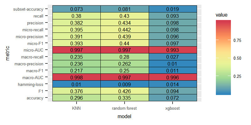
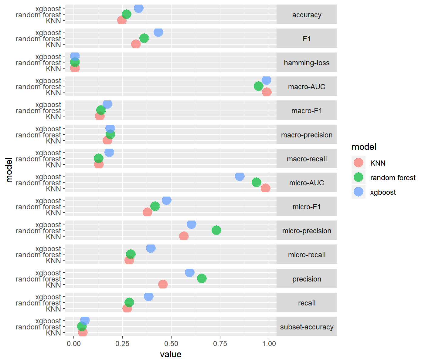
For the purpose of the evaluation task, The mldr package equipped us with multilabel_evaluate method to inspect many evaluation metrics(accuracy, micro based metrics, macro based metrics, precision, recall, F1, subset-accuracy). We will present all of them for each experiment. Through the exploration process of the Eur-Lex dataset, we come to know the class labels are imbalanced (i.e. some labels are frequent and some are infrequent). In that case considering accuracy is a misleading measure of the performance, instead we consider F1 as a comparision factor among the classifiers. Infact we consider macro-F1 as the Macro-average will compute the metric independently for each class and then take the average (hence treating all classes equally), which is desirable in case of class imbalance.
Dataset: English
This section answers three research questions for the English corpus:
- How well the classifiers perform over Eur-Lex dataset?
- How the classifiers’ performance changes with different features- one with term frequency-inverse document frequency(tf-idf), another with term incidence?
- Which flavour of multilabel transform algorithm perform best among all, the one which considers label correlation or the one which does not?
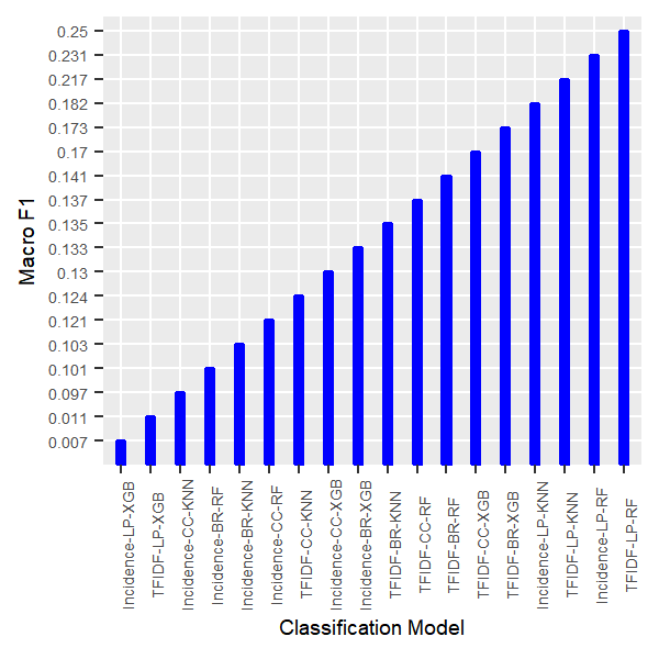
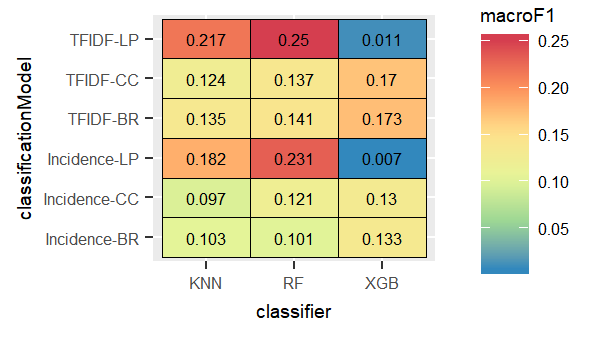
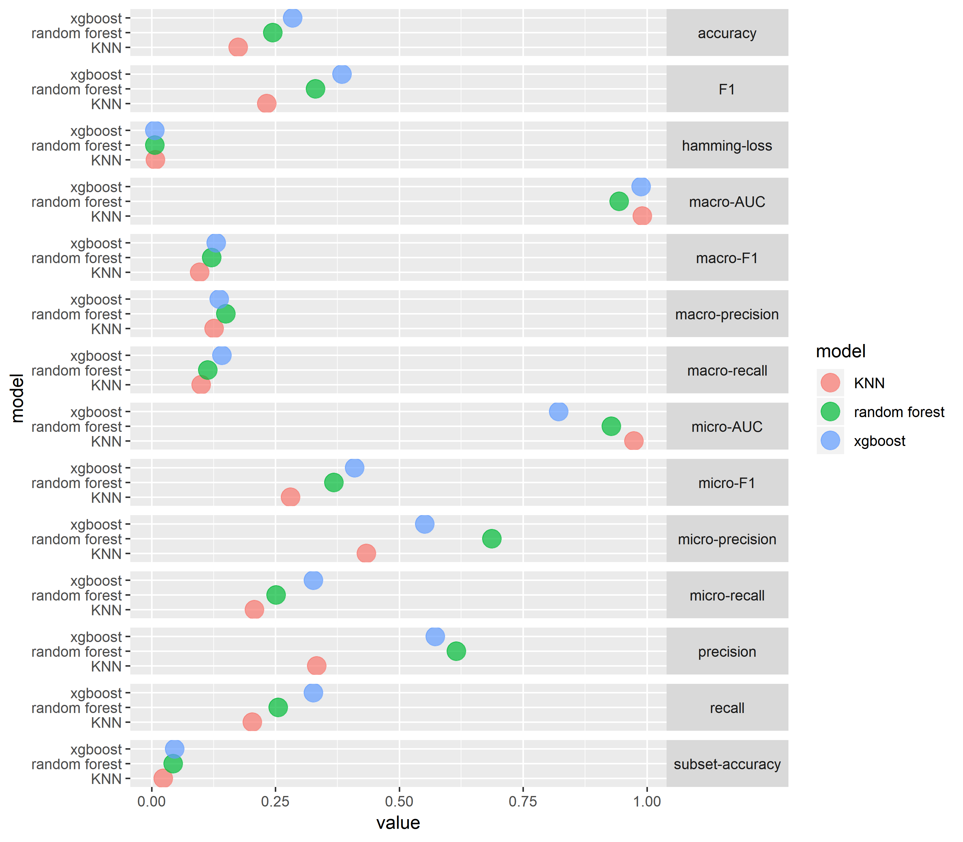
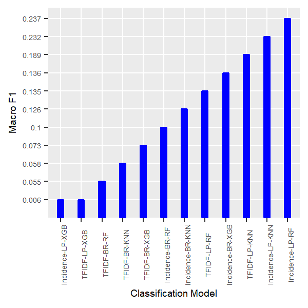
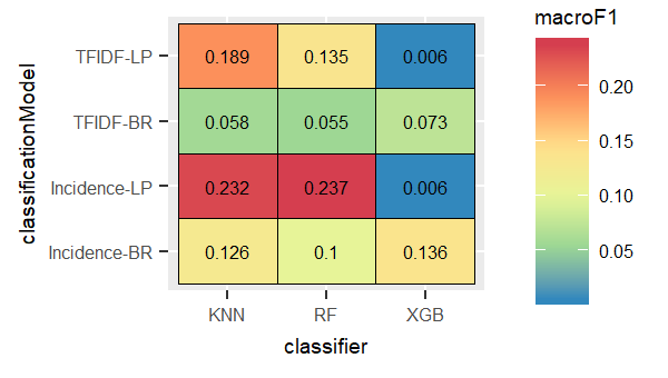
For the English dataset, we observed higher macro F1 over all the nine trained classifiers when we used tf-idf as the features. Tf-idf is more powerful representative features than simply using the incidence of terms as features. The expreiments portrayed that LP combined with the Random Forest recorded the best result for the two type of features(tf-idf and term incidence), whereas the LP method combined with XGB performed the worst as shown in the following figures:
In the following sections we will display the results in detail for each dataset.
Dataset: English, Feature: Tf-idf
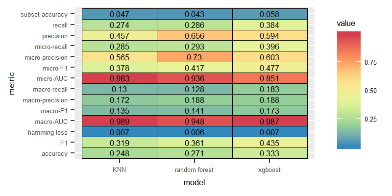
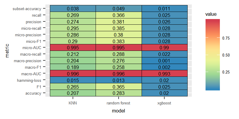
Label Powerset
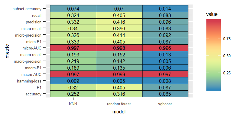
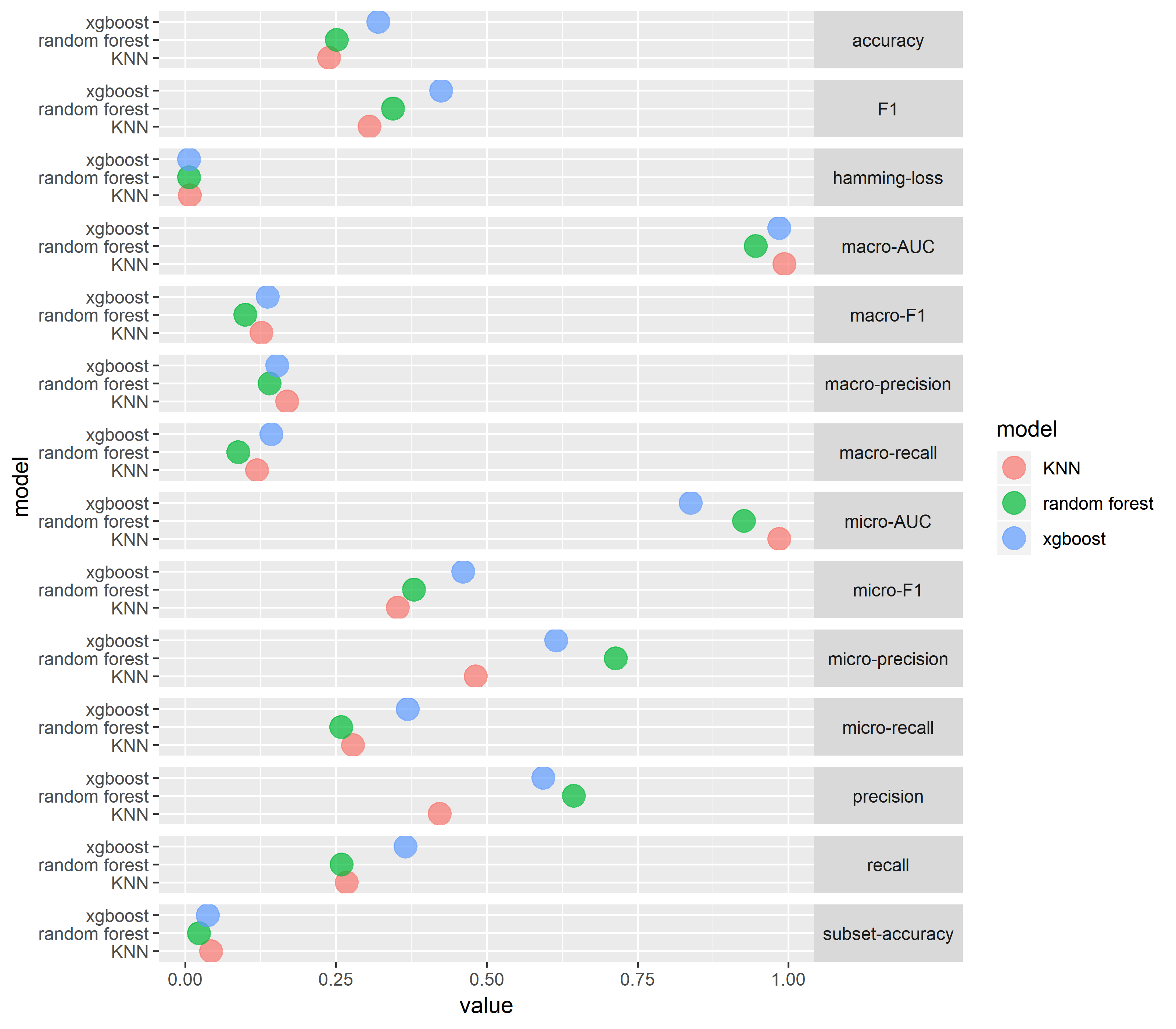
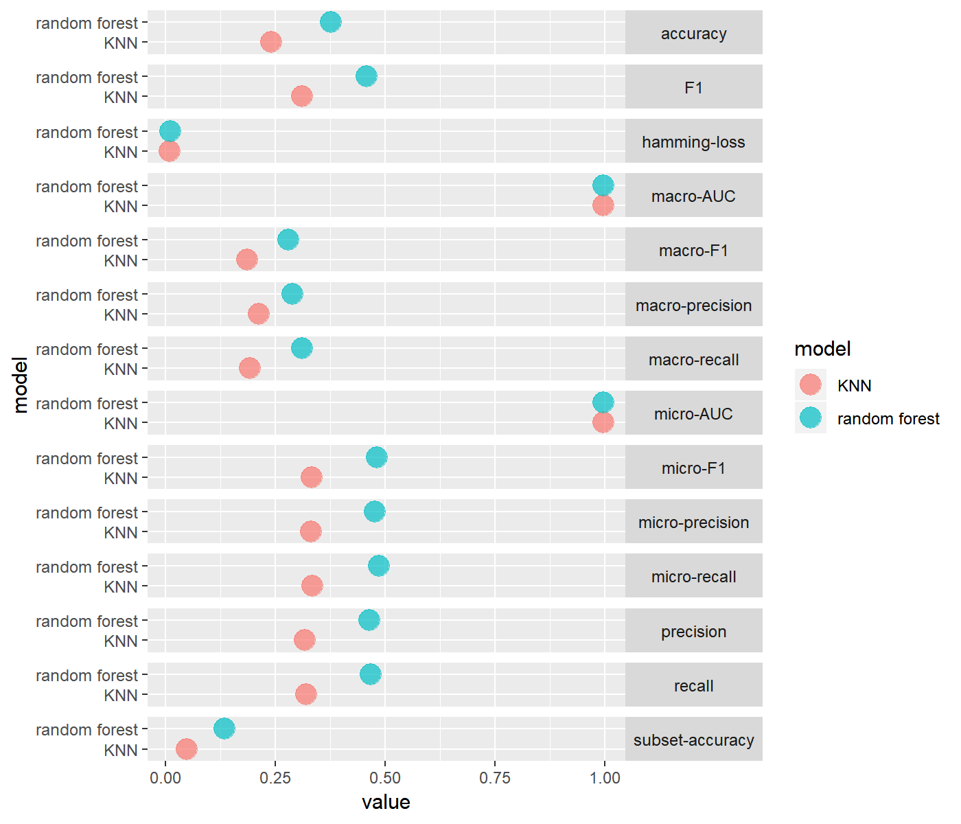
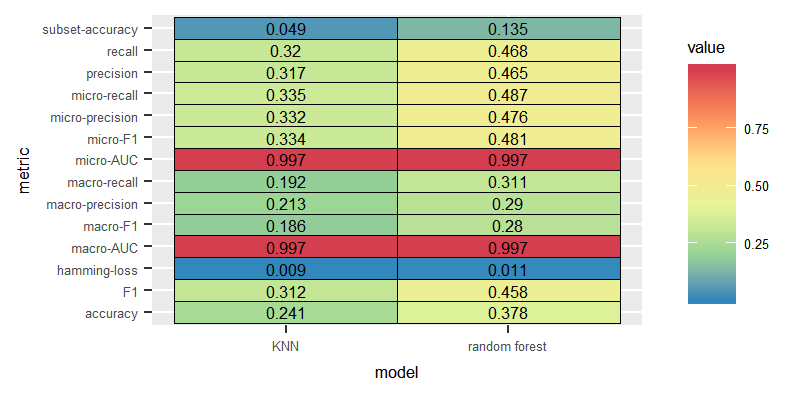
According to the following figures, LP with KNN and Random Forest performed the best, and XGBoost performed the worst.

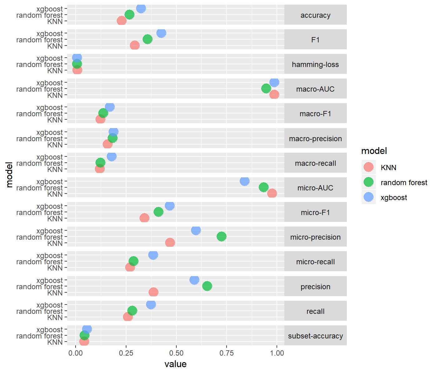
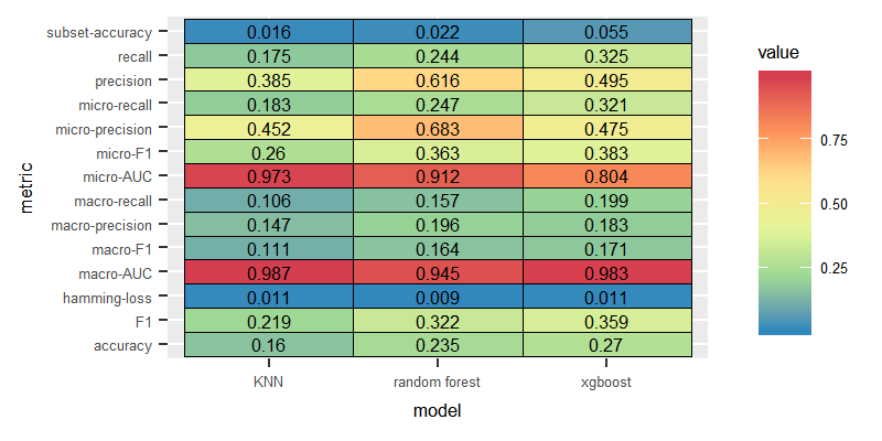
Binary Relevance
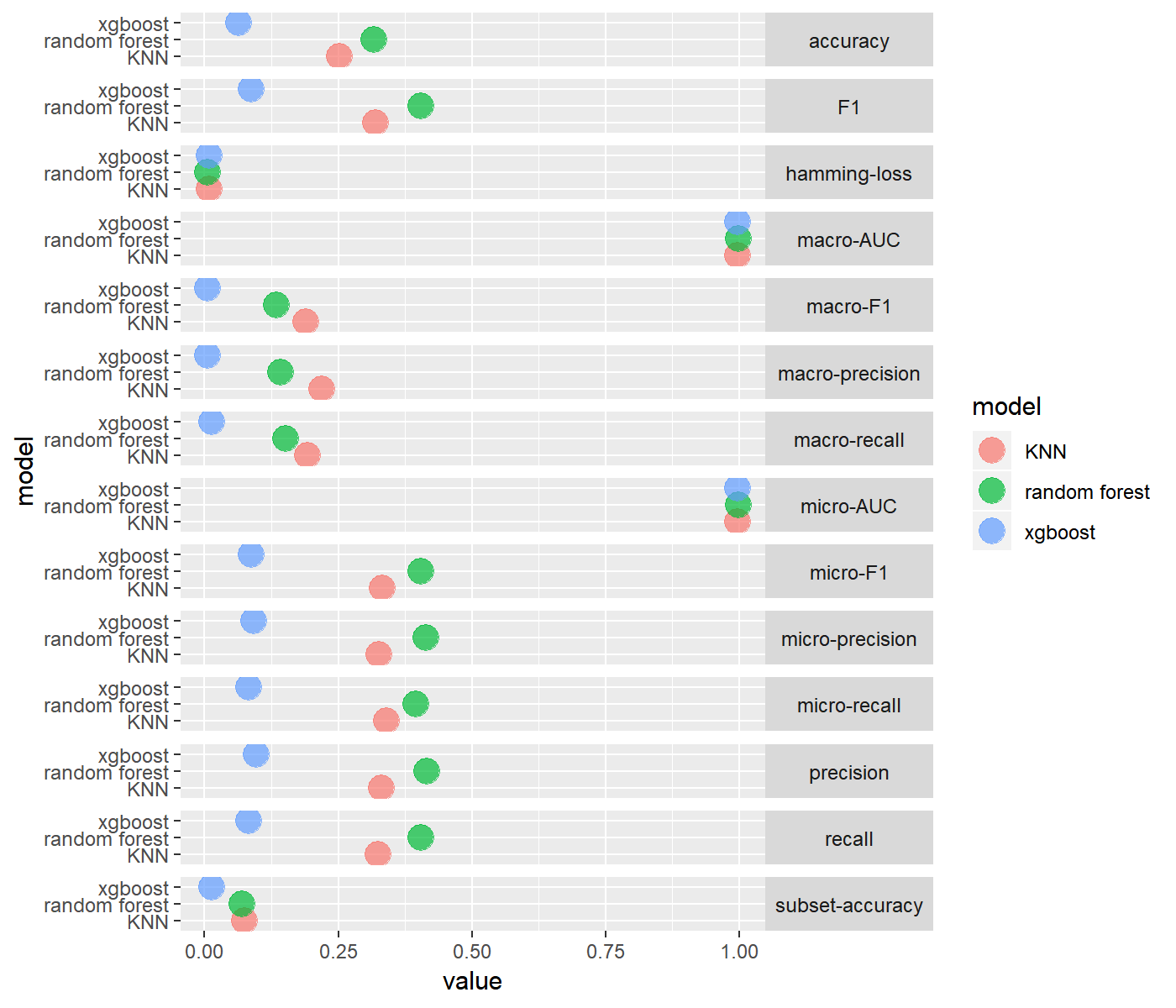
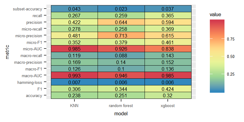
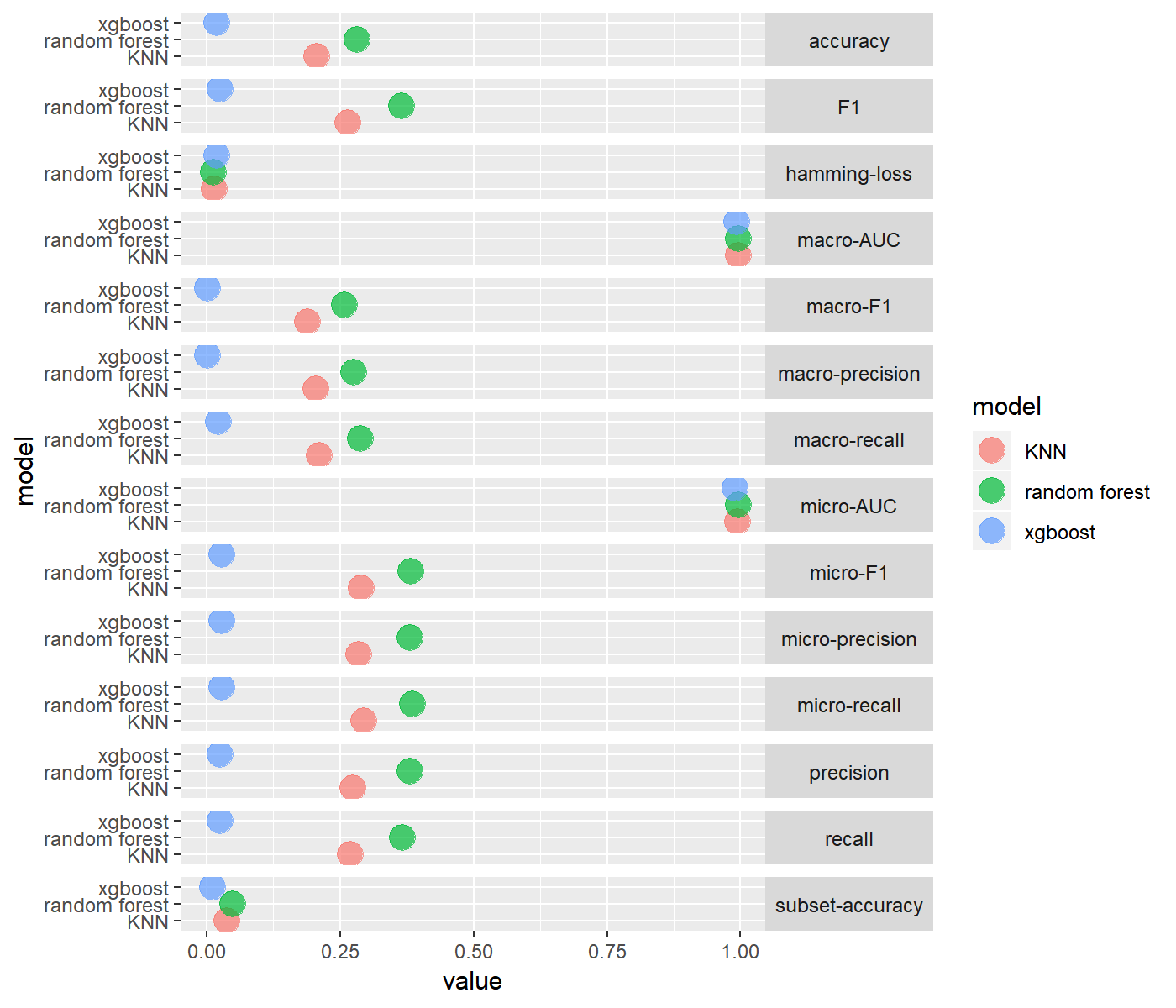
We compared the three models where the labels are assumed to be independent. The BR method produced the best results when combined with XGBoost.
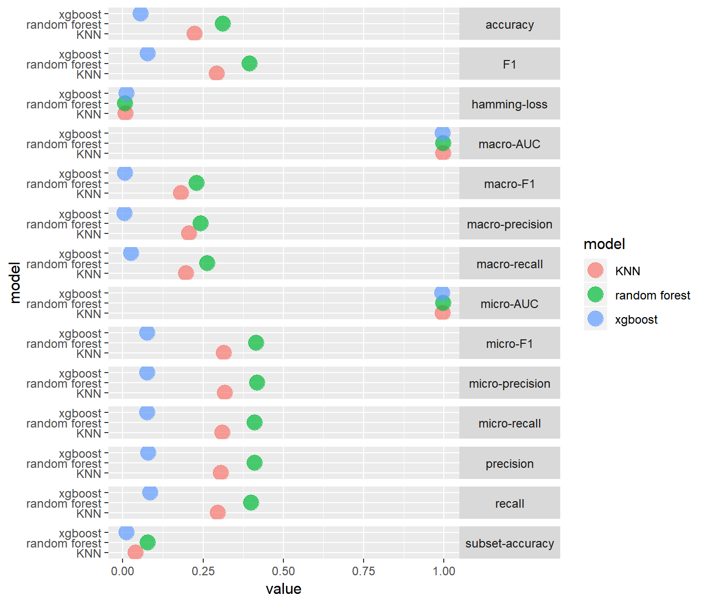
Classifier Chain
Similar to the BR method, CC method performed the best with the XGBoost classifier.

Dataset: English, Feature: Term incidence
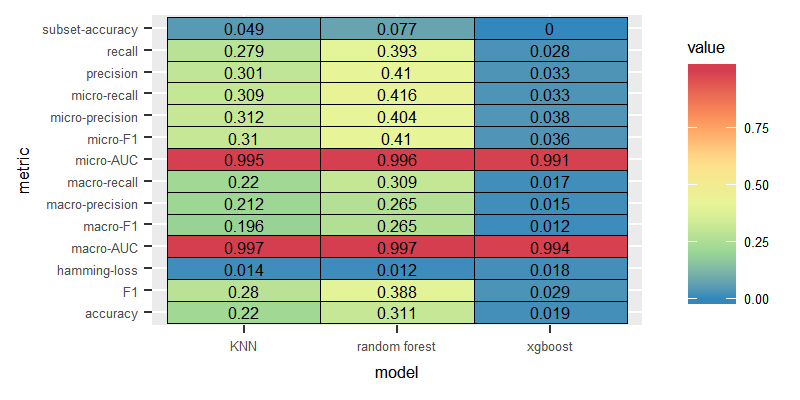
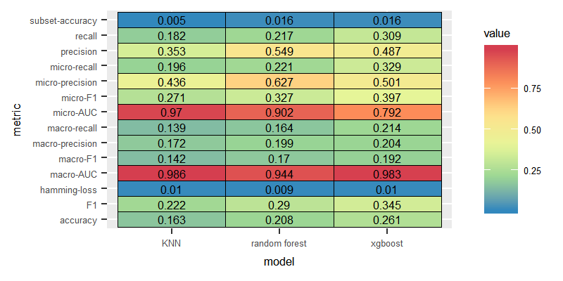
We wanted to test the performance of the models in case of employing more naive features as the incidence of terms. The experiments showed similar pattern to the experiments with tf-idf dataset-LP with the Random Forest scored the highest macro F1 value, with the XGBoost performing the worst. Nevertheless, classifiers trained on the incidence of terms as features did not score better than the ones trained on the tf-idf features.
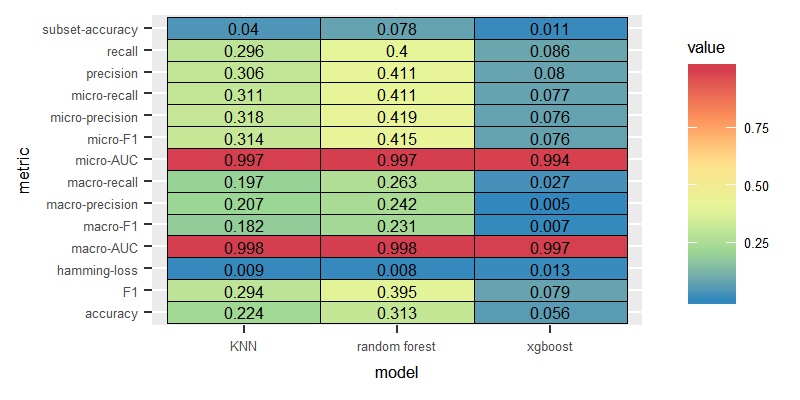
Label Powerset
Binary Relevance


Classifier Chain

Dataset: German
This section answers three research questions for the English corpus:
- How well the classifiers perform over Eur-Lex dataset?
- How the classifiers’ performance changes with different features- one with term frequency-inverse document frequency(tf-idf), another with term incidence?
- Which flavour of multilabel transform algorithm perform best among all, the one which considers label correlation or the one which does not?
Similar to the experiments run over the English dataset, for the German dataset the experiments showed that LP combined with Random Forest or KNN recorded the best results for the two type of features(tf-idf and incidence of terms), compared to the low performance produced by the LP method combined with XGBoost. On the other hand, in the contrast to the results for the English dataset,for the German dataset, we observed higher macro F1 over all the nine trained classifiers when we used incidence of terms instead of the tf-idf as features.
In the following sections we will display the results of the experiments run on the German dataset in detail for each type of features.
Dataset: German, Feature: Tf-idf
Unlike the experiments conducted on the English dataset, LP combined with KNN delivered slightly higher performance than the model combining the LP with Random Forest.
Label Powerset
Binary Relevance
The performance of BR was significantly poor over the three models. 

Dataset: German dataset, Feature: Incidence of terms
The classifiers performed better over term incidence features, which portrays term incidence are good discriminatory features compared tf-idf, which demands more computational effort compared to term incidence.
Label Powerset


Binary Relevance
Dataset with balanced labelsets
Training our classification models on a dataset with such a large number of labels(7000 labels) was a challenging task. we surmised that reducing the number of labels would improve the predictive capacity of the classifiers. To reduce the large number of labels, we take advantage of the “scumble” attribute provided by the mldr package. Scumble measure indicates the concurrence level among frequent and infrequent labels in the same labelsets. we simply removed imbalanced labelsets(i.e imbalanced labelsets are labelsets with frequent and infrequent labels) and kept only balanced labelsets by filtering only labelsets with lower level of scumble values than the mean scumble value of the dataset with the following command line:
datasetWithBalancedLabelsets <- dataset[.SCUMBLE <= dataset$measures$scumble]Dataset: English, Balanced labelsets
This section the answers research question for the English corpus:
How the classifiers’ performance changes when the number of labels is reduced, and which features delivered the best performance.
Some classifiers scored higher than the highest macro F1 value scored in the case of keeping imbalanced labelsets. Employing the tf-idf features yielded higher macro F1 for classifiers trained on the complete set of labels. In the case of balanced labelsets, classifiers trained on the incidence of terms showed slightly better performance as shown in the following graphs:


Dataset: English, Feature: Tf-idf, Balanced labelsets
For the tf-idf features, most of the classifiers trained on the balanced labelsets maintained almost similar levels of performance compared to the performace with the complete set of labels.
Label Powerset
Binary Relevance

Dataset: English, Feature: Term incidence, balanced labelsets
For balanced labelsets, we observed better performance for the incidence features for all classifiers compared to the performance with the complete labelsets. LP combined with the Random Forest classifier outperformed the performance of the same classification model trained on the complete set with the tf-idf features. We consider incidence of terms as sufficient features even for the English dataset, after pruning the imbalanced labelsets.
Label Powerset

Binary Relevance

Dataset: German, Balanced labelsets
This section answers the research question for the German corpus:
How the classifiers’ performance changes when the number of labels is reduced, and which features delivered the best performance.

Dataset: German, Feature: Tf-idf, Balanced labelsets
After removing the imbalanced labelsets, the macro F1 for the combination of LP with Random Forest increased by around 15%.
Dataset: German, Feature: Term incidence, balanced labelsets

Final Analysis
We can conclude for both English and German dataset,the best performance was delivered by the LP transform combined with the Random Forest classifier after removing imbalanced labelsets through exploiting the scumble measure and trained on the terms incidence in order to gain the highest macro F1 values.
Based on the results of various experiments that we conducted on the different classification models, the best performance was observed for the combination LP transform with Random Forest and LP transform with K-nearest neighbour, compared to BR transform along with the same classifiers .
As mentioned earlier, LP transform takes into consideration the correlation among the labels. In contrast, the BR transform assumes the labels to be independent and ignores any dependency among labels. We infer that the assumption of the independency of labels does not hold in the case of the EUR-Lex dataset.
Contrary to the LP method,each model in the BR transform considers the labels independently- it reduces the number of labels when applying the BR to build an independent classifier for each label, which improves the perfomance of the XGBoost classifier by the model optimization technique the XGB follows.
In experiments over the BR transformation method, XGBoost performed better than the Random Forest and the k-nearest neighbour classifiers. We surmise, since XGBoost classifier is an ensemble model uses “Boosting” as a deliberate ensemble technique, whereas Random Forest employs “Bagging” as an ensemble technique and KNN encounters the curse of dimensionality.
CC transform method delivered poor performance across all classication models(k-nearest neighbour, Random Forest, XGBoost). XGBoost performed the best with CC, due to the boosting optimization technique the XGBoost based on.
Suprisingly, we found the classifiers trained on the terms incidence features performed better than when trained on the tf-idf features. we think that the occurance of the term in a document was a sufficient distinctive feature of the documents of the legal EUR-Lex dataset.
With balanced labelsets we found that the classifiers overall performed better, though not much, for both English and German dataset.
Conclusion
The best score for macro-F1/F1 we could get for the English dataset is 0.265/0.365 and for German dataset is 0.269/0.458, and the publications using the earlier version of the dataset having 4000 labels also reported a poor F1 score less than 0.5. It implies that the features which we have used might not have behaved as discriminatory as expected, but we cannot rule out the bias of the annotators, which might have prevented us to get good results. The annotators categorizing the document might have been influenced by various aspects as mentioned in literature [1] while assigning them to the categories. Therefore it seems challenging for the machine learning algorithms to match with the human annotated categories.
References
1. Räbiger S, Spiliopoulou M, Saygına Y. How do annotators label short texts? Toward understanding the temporal dynamics of tweet labeling. 2018.