Exploratory analysis
This section deals with the exploratory analysis for the English EUR-Lex dataset. Exploratory analysis over German corpus can be found in the GitHub repository
Dataset
The Eurlex dataset for every language comprises two files- a cf file and a XML file.
The documents(laws/treaties) and the document categories/labels is available in the cf file (acquis.cf). The content and the labels for each document has been stored in the file in the following way:
- Every odd line consists of label-ids and the document-id of a document. The labels and document-id is separted by a #.
- Every even line consists of the actual text.
An example has been shown below in the diagram below. On the 1st line there are two lable-ids - 3032, 525 and the document-id is 31958d1006(01), and the actual text is on 2nd line.
![[Fig1. Data format]](Figs/acquis.png)
The mapping between label-id and label-name has been provided in a XML. A small snippet of the xml has been provided below.
<?xml version="1.0" encoding="UTF-8" ?>
<!DOCTYPE DESCRIPTEUR SYSTEM "descripteur.dtd">
<DESCRIPTEUR LNG="EN" VERSION="4_3">
  <RECORD>
    <DESCRIPTEUR_ID>4444</DESCRIPTEUR_ID>
    <LIBELLE>abandoned land</LIBELLE>
  </RECORD>
</DESCRIPTEUR>
The tag DESCRIPTEUR_ID contains the label-id and LIBELLE contains the label name.
Text Preprocessing
For our task two kinds of preprocessing is needed:
Text preprocessing
Text data contains many characters which do not convey much information, like punctuations, white spaces, stop words, etc. In English, certain words like “is”, “the” is present in every document and does not help to discriminate two documents. But again, depending on the language and the task at hand, we need to deal with such characters differently.Preprocessing to generate the data expected by mldr
To study the MLD datasets traits (label distribution, relationship among labels and label imbalance) and perform classification over MLD datasets we need to transform the available dataset into mldr format - a sparse ARFF file containing features and labels , and a XML file containing the label names.
How much the preprocessing varies across languages for our task?
Preprocessing will be almost same for both languages - English and German, except for the following:
- list of stopwords
- lemmatization - The lemmatization for English language could be done using the method lemmatize_strings from package textstem, but for German language we had to use udpipe model.
Features used for the task
We will be using two sets of features - term incidence and tf-idf as features, and will try to answer the research question - “How the classifiers’ performance changes with different features- one with term frequency-inverse document frequency(tf-idf), another with term incidence?”
Therefore we will have two datasets/ARFFs for each language- one containing term-incidence as features and the other containing tf-idf as features.
Since the pre-processing is little different for different languages, we need to execute the following code, to perform the pre-processing for a particular language.
library(udpipe)

init <- function(language) {
  if (language == "english") {
  print("english chosen")
    lang <<- "english" # language chosen - english
    fileName <<- "../data/english/acquis.cf" # file containing data (english)
    tfidfFileName <<- "../output/tfidf_EN" # tf-idf arff file (english)
    incFileName <<- "../output/inc_EN" # term incidence arff file (english)
    labelFile <<- "../data/english/desc_en.xml" # label-names file (english)
  }
  else if (language == "german") {
  print("german chosen")
    lang <<- "german" # language chosen - german
    fileName <<- "../data/german/acquis_german.cf" # file containing data (german)
    tfidfFileName <<- "../output/tfidf_DE" # tf-idf arff file (german)
    incFileName <<- "../output/inc_DE" # term incidence arff file (german)
    labelFile <<- "../data/german/desc_de.xml" # label-names file (german)
    model_file <<- "../output/german-gsd-ud-2.3-181115.udpipe" # udpipe german model for lemmatization
    if (!file.exists(model_file))
    { #
      model <<- udpipe_download_model(language = "german", model_dir = "../output/")
    } else {
      model <<- udpipe_load_model(model_file)
    }
  }
}
We need to pass “english” for English text and “german” for German text in the method init(). We will be performing exploratory analysis for English legal text, therefore passing english.
#Choosing english for preprocessing
init("english")
## [1] "english chosen"In the text preprocessing we need to preprocess two things - the actual text and the labels.
Lemmatization using udpipe model needs to be done in small batches of documents, else we get a weird exception when the document size exceeds a limit, therefore we need to define the following function:
#generates lemma for each german document
generate_lemma_per_document <- function(content, doc_id) {
  annotated_data_table <-
  udpipe_annotate(
  model, #udpipe german model
  x = content, #character vector in UTF-8 encoding
  doc_id = doc_id, #document-id
  tagger = "default", #default udpipe POS tagging and lemmatisation
  parser = "none" #no dependency parsing needed
  ) %>% as.data.table() #generate data table

  lemma <- sapply(annotated_data_table$lemma, paste, collapse = " ") #extract lemma from data table
  return(lemma)
}
The following method performs the preprocessing for the actual text.
library(textstem)
library(textclean)
library(tm)

#generates clean text
get_clean_content <- function(content) {
  clean_content <- content  %>%
    replace_html(replacement = " ") %>%       #replace html tags with space
    { gsub('-', '', .) } %>%                  #removes hyphen between words
    { gsub('[[:punct:] ]+', ' ', .) } %>%     #removes punctuations
    { gsub("\\b[IVXLCDM]+\\b", " ", .) } %>%  #removes roman numerals
    tolower()                                 #to lower case

  if (lang == "english"){   # lemmatization for english
    clean_content <- lemmatize_strings(clean_content)

  } else {  # lemmatization for german
    lemmata <- c()
    for (index in 1:length(clean_content)) {
      lemmata[index] <-
        mclapply(
          clean_content[[index]], FUN = function(x)
            generate_lemma_per_document(x, index) #generate lemma for each document
        )
    }
    clean_content <- sapply(lemmata, paste0, collapse = " ") #append generated lemmata for each document
  }

  clean_content <- clean_content %>%
    removeNumbers() %>%                       #removes numbers
    removeWords(words = stopwords(lang))  %>% #removes stopwords
    replace_non_ascii(replacement = " ")  %>% #removes non-ascii terms
    trimws()                                  #removes extra space

  clean_content
}
We will now load the text for the selected language by init(), and inspect the 1st document’s content.
library(dplyr)

connection <- fileName  %>% file(open = "r")
raw_text_char <- connection %>% readLines(encoding = "UTF-8")
close.connection(connection)
text_content_list <-
raw_text_char[seq (2, length(raw_text_char), 2)] #every even line contains text

text_content_list[[1]] #1st document's content
## [1] "<P>DECISION creating the \"Official Journal of the European Communities\"</P> <P>THE COUNCIL OF THE EUROPEAN ECONOMIC COMMUNITY,</P> <P>Having regard to Article 191 of the Treaty establishing the European Economic Community; Having regard to the proposals from the President of the European Parliament and the Presidents of the High Authority, the Commission of the European Economic Community and the Commission of the European Atomic Energy Community; </P> <P>Whereas the European Economic Community, the European Coal and Steel Community and the European Atomic Energy Community should have a joint official journal; </P> <P></P> <P>HAS DECIDED:</P> <P></P> <P>to create, as the official journal of the Community within the meaning of Article 191 of the Treaty establishing the European Economic Community, the Official Journal of the European Communities.</P> "After loading the text, we preprocess it.
text_content_list <- get_clean_content(text_content_list)Let’s inspect the same (1st) document’s preprocessed content.
text_content_list[[1]]## [1] "decision create official journal european community council european economic community regard treaty establish european economic community regard proposal president european parliament president high authority commission european economic community commission european atomic energy community whereas european economic community european coal steel community european atomic energy community joint official journal decide create official journal community within mean treaty establish european economic community official journal european community"We need to preprocess labels, as label names are in different file. The dataset- acquis.cf file just contains label-ids. Also the label names contains certain characters like space which is inconvenient to generate MLD datasets.
The following code generates clean label name for all documents.
# get clean labels
get_clean_label <- function(labels) {
  labels <- labels %>%
  {
  #replace certain characters with hyphen
  gsub("\\s|\\.|\\[|\\]|-|\\(|\\)", "_", .)
  } %>%
  {
  #remove quotes
  gsub("'", "", .)
  } %>%
  replace_non_ascii(replacement = " ") %>% #remove non-ascii characters
  tolower()  %>% #to lower case
  paste("_", sep = "") #append hyphen at the end

  labels
}
The below utility method retrieves the label name.
get_label_name <- function(label_id, label_id_name_df) {
  label_name = label_id_name_df[label_id_name_df$did == label_id, 2]
  if (length(label_name) > 0)
    return(as.character(label_name))
  else
    return(paste(label_id, "_" , sep = "")) #some label-ids don't have mapping in xml
}
We need to create a dataframe from the label id-name mapping xml. we will use the dataframe to retrieve the label-names from the label-ids.
library(XML)

# gets label name from label-id using xml, [594 4444] -> [AAMS countries abandoned land]
get_label_name_list <- function(label_id_list) {
  desc_xml <- xmlParse(labelFile)

  # a dataframe containing label-id and label-name
  xm_df <-
    data.frame(did = sapply(desc_xml["//DESCRIPTEUR_ID"], xmlValue),
               dname = sapply(desc_xml["//LIBELLE"], xmlValue))

  xm_df$dname <- get_clean_label(xm_df$dname)

  label_name_list <- label_id_list %>%
    lapply(function(labelsets)
      strsplit(labelsets, " ")) %>% # split the label-ids (594 4444)
    sapply("[[", 1) %>%  # get each array elements- list of list of label-ids
    lapply(function(label_id_array)
      lapply(label_id_array, function(label_id)
        # get label-name for each label-id in the list
        get_label_name(label_id, xm_df))) %>%
    lapply(function(label)
      paste(label, sep = " "))  # append the label-names (AAMS countries abandoned land)

  label_name_list
}
After defining the utility methods for label preprocessing we will load and generate the clean label list.
class_labels_list <-
  raw_text_char[seq (1, length(raw_text_char), 2)] %>% #every odd line contains labelsets for the document
  strsplit("#") %>%
  sapply("[[", 1) %>%
  trimws() %>%
  get_label_name_list()
After generating a cleaner version of text and labels we can take a deep dive into the first part of our data exploration.
Data Exploration
We have now a list of document content and a list of labelsets (list of labels for one document). To perform exploratory analysis we need to generate a dataframe containing the text and one corresponding label (instead of labelsets) against each document.
text <- character()
label <- character()
for (index in 1:length(text_content_list)) { #iterate over all documents
  temp_labelset <- unlist(class_labels_list[[index]]) #unlist the label-list for the document
  for (label_index in 1:length(temp_labelset)) #iterate over all labels for the document
  {
    text <- append(text, text_content_list[[index]])
    label <- append(label, temp_labelset[[label_index]])
  }
}

#generate dataframe from list of text and label
text_df <- as.data.frame(cbind(text, label), stringsAsFactors = FALSE)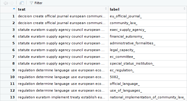
Wordcloud
We start exploration with wordcloud, which is a simple yet informative way to understand textual data and perform analysis. We need to generate tokens and count the frequency of words, to generate the word cloud.
library(tidytext)

tokens <- text_df %>%
  unnest_tokens(word, text) %>%
  dplyr::count( word, sort = TRUE) %>%
  ungroup()
Now we generate word cloud.
library(wordcloud)

wordcloud(words = tokens$word, freq = tokens$n, min.freq = 1, max.words=50, random.order=FALSE, rot.per=0.35,colors=brewer.pal(8, "Dark2"),scale=c(3.5,0.25))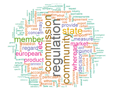
The prominent words popping in the wordcloud are all law related terms like - “regulation”, “commission”, which does not give us any helpful insight. Therefore we need to incorporate certain law related stopwords in our preprocessing. We remove those stopwords from our dataframe and generate the wordcloud again.
law_stopwrds <- c("gt","notext","p","lt","aka","oj","n","a","eec","article","directive","shall","follow", "accordance","chairman","necessary","comply","reference","commission","opinion","decision","annex","refer","member","european","treaty","throughout","regulation","particular","thereof","community","committee","measure","parliament","regard","amend","procedure","administrative","procedure","publication","month","date","year","enter","force","ensure","authority","take","council","act","within","national","law","main","provision","mention","approve","certain","whereas","eea","also","apply","may","can","will","shall","require","paragraph","subparagraph","official","journal","article","ec","b","s","c","e")

tokens <- tokens[!tokens$word %in% law_stopwrds, ]

wordcloud(
  words = tokens$word,
  freq = tokens$n,
  min.freq = 1,
  max.words = 50,
  random.order = FALSE,
  rot.per = 0.35,
  colors = brewer.pal(8, "Dark2"),
  scale = c(3.5, 0.25)
  )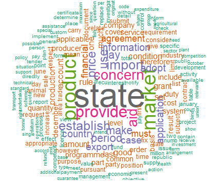
The wordcloud generated now gives more informative insight. It seems the documents/laws are related to state more than a country. Also appearance of certain terms like “export”, “import”, “aid”,“financial”, “grant”, makes it appear that many documents are related to import-export and financial aids/grants.
Term frequency
After getting some insight from the wordcloud we examine it further. It will be interesting to see which terms are common for different category of legal text. To get that, we need to count words for each category.
tokens_by_label <- text_df %>%
  unnest_tokens(word, text) %>% #generate tokens
  dplyr::count(label, word, sort = TRUE) %>% #counts words for each category
  ungroup()

total_words <- tokens_by_label %>%
  group_by(label) %>%
  summarize(total = sum(n)) # sum of words' count for each category

tokens_by_label <- left_join(tokens_by_label, total_words) #add total count column (total) to the data frame

tokens_by_label 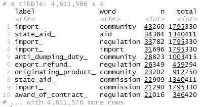
There is one row in the data frame tokens_by_label for each word-label combination. n is the number of times that word is used in that legal text category/label and total is the total words in that category. Let us have a look at the distribution of (n/total) for each document category- the number of times a word appears in a label divided by the total number of terms in that category. Our dataset has around 7000 labels , and it will be difficult to analyse over all categories! Therfore, we will consider some of the categories for our analysis.
library(ggplot2)

tokens_by_label %>% filter(
  label == "water_treatment_" |
  label == "wastewater_" |
  label == "pollution_control_" |
  label == "atmospheric_pollution_" |
  label == "fight_against_unemployment_"
  ) %>%
  ggplot(aes(n / total, fill = label)) +
  geom_histogram(show.legend = FALSE) +
  xlim(NA, 0.0009) +
  facet_wrap( ~ label, ncol = 2, scales = "free_y")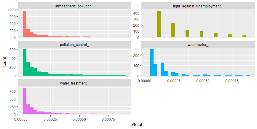
We observe there are very long tails to the right for the categories portrayed above in the picture. Distributions like those shown in the figure above are very common in any given corpus of natural language -website, books, etc, and portrays that there are many words that occur rarely and fewer words that occur frequently. We can use the term frequency dataframe to plot term frequency and examine Zipf’s law.
Zipf’s law states that the frequency that a word appears is inversely proportional to its rank.
#generate term frequency for each category
freq_by_rank <- tokens_by_label %>%
  group_by(label) %>%
  mutate(rank = row_number(),
  `term frequency` = n / total)

# generate Zipf's law graph
freq_by_rank %>%
  ggplot(aes(rank, `term frequency`, color = label)) +
  geom_line(size = 1.1,
  alpha = 0.8,
  show.legend = FALSE) +
  scale_x_log10() +
  scale_y_log10()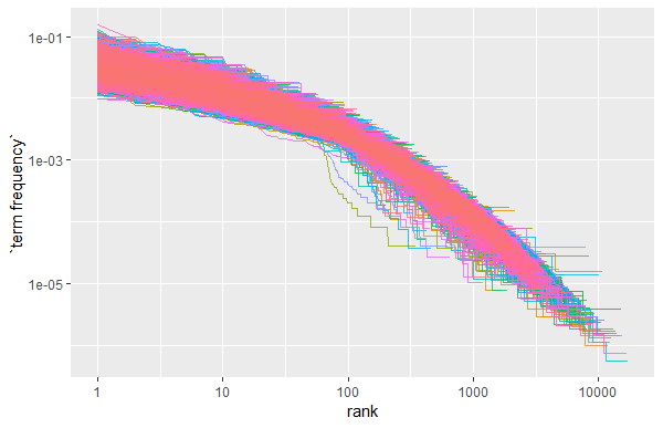
The above plot is in log-log coordinates. We can see that all the document categories in the corpus exhibit similar behaviour, and the relationship between rank and frequency does have negative slope, implying that they follow Zipf’s Law.
Top k words
It would be interesting to find out top 10 words for each category, which will give us an idea what each category of law document deals with. To find the most importants words it would make sense to use tf-idf rather than term frequency, as tf-idf finds the important words for the content of each document category by decreasing the weight for commonly used words and increasing the weight for words that are not used very much in a collection or corpus of documents.
tokens_by_label <- bind_tf_idf(tokens_by_label, word, label, n) #generates tf-idf and binds to dataframe
tokens_by_label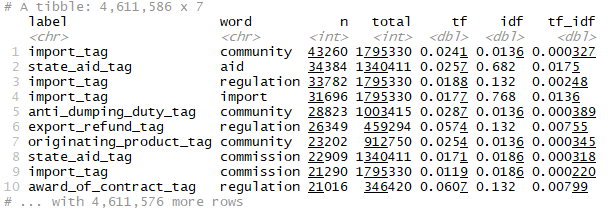
Generating the top-10 words’ plot now.
tokens_by_label %>%
  filter(
  label == "water_treatment_" |
  label == "wastewater_" |
  label == "pollution_control_" |
  label == "atmospheric_pollution_" |
  label == "fight_against_unemployment_"
  ) %>%
  arrange(desc(tf_idf)) %>%
  mutate(bigram = factor(word, levels = rev(unique(word)))) %>%
  group_by(label) %>%
  top_n(10) %>%
  ungroup %>%
  ggplot(aes(word, tf_idf, fill = label)) +
  geom_col(show.legend = FALSE) +
  labs(x = NULL, y = NULL) +
  facet_wrap( ~ label, ncol = 2, scales = "free") +
  coord_flip()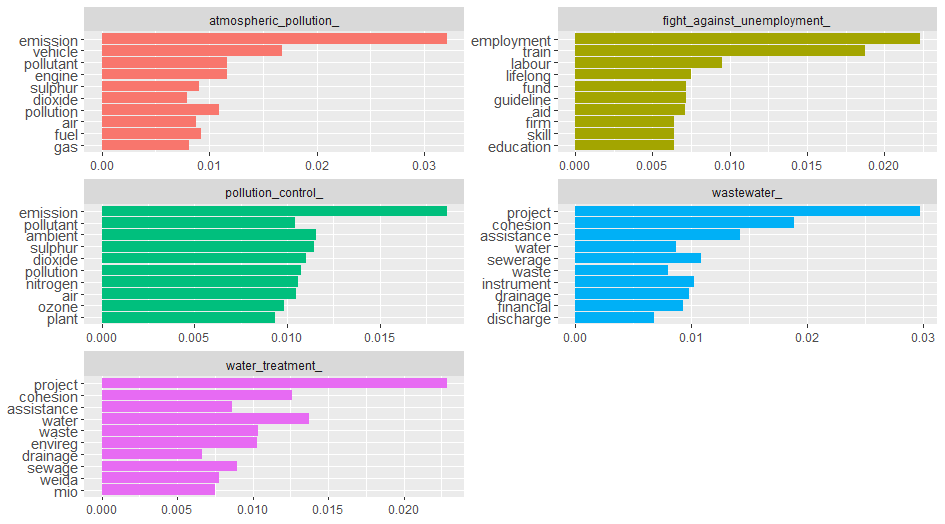
We can see from the above figure the categories/labels - atmospheric_pollution_, pollution_control_ share many common words which implies a lot of pollution related documents are dealing with air pollution. There are many common terms among documents wastewater_ and water_treatment_ as expected, as both deal with waste water. The category fight_against_unemployment_tag does not share any common terms with the other categories. Actually it would have been interesting if it would have happened! - which would have implied that employment/unemployment might have resulted from pollution or water related cause.
Sometimes bigrams are more meaningful than single words, and it would be interesting to see how the top 10 words changes for bigrams.
Top k bigrams
We generate the tokens in similar way, except we use we used token = “ngrams” and n=2 in the method unnest_tokens.
#generate bigram tokens
bigram_tokens <- text_df %>%
  filter(grepl('water|pollution|employment', label)) %>%
  unnest_tokens(bigram, text, token = "ngrams", n = 2) %>%
  dplyr::count(label, bigram, sort = TRUE) %>%
  ungroup()

total_words <- bigram_tokens %>%
  group_by(label) %>%
  summarize(total = sum(n))

bigram_tokens <- left_join(bigram_tokens, total_words)
bigram_tokens <- bind_tf_idf(bigram_tokens, bigram, label, n)

#generate top 10 bigram plot
bigram_tokens %>%
  filter(
  label == "water_treatment_" |
  label == "wastewater_" |
  label == "pollution_control_" |
  label == "atmospheric_pollution_" |
  label == "fight_against_unemployment_"
  ) %>%
  arrange(desc(tf_idf)) %>%
  mutate(bigram = factor(bigram, levels = rev(unique(bigram)))) %>%
  group_by(label) %>%
  top_n(10) %>%
  ungroup %>%
  ggplot(aes(bigram, tf_idf, fill = label)) +
  geom_col(show.legend = FALSE) +
  labs(x = NULL, y = NULL) +
  facet_wrap( ~ label, ncol = 2, scales = "free") +
  coord_flip()
We can see again the categories pollution_control_tag and atmospheric_pollution_tag share most of the bigrams, and similarly water related categories share many bigrams. fight_against_unemployment_tag category again stands alone and does not share any common bigrams with other categories in the plot.
Word association
Another way to view word connections is to treat them as a network, similar to a social network. Word networks show term association and cohesion. In a network graph, the circles are called nodes and represent individual terms, while the lines connecting the circles are called edges and represent the connections between the terms. We can see some interesting word association in the figure below.
library(tidyr)
library(igraph)
library(ggraph)

(
  bigram_graph <-
  bigram_tokens %>% dplyr::count(bigram, sort = TRUE) %>% #count bigram occurence
  top_n(100) %>% #select top 100 frequent bigrams
  graph_from_data_frame() #generate graph from dataframe
  )

  #generate word network graph
  ggraph(bigram_graph, layout = "fr") +
  geom_edge_link() + #draws edges between nodes
  geom_node_point(color = "lightblue", size = 5) + #assign colour and size to nodes of graph
  geom_node_text(aes(label = name), vjust = 1, hjust = 1, check_overlap = TRUE) + #adjusts text in graph
theme_void() 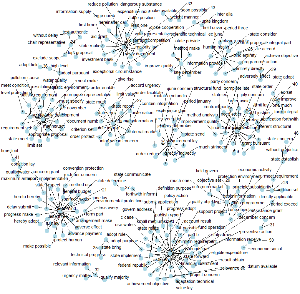
Preprocessing for mldr
To perform the exploratory analysis over the multilabel (MLD) dataset traits we need to generate the dataset in the format which can read by mldr package, as discussed in this section. Since our objective in performing exploratory analysis over the multilabel dataset is to inspect certain multi-label dataset traits (label distribution, relationship among labels and label imbalance), it is fine if we perform the analysis over one of the datasets (tf-idf or incidence). Therefore we generate one of the datasets for exploratory purpose. We generate the tf-idf dataset.
First we generate VCorpus and then DocumentTermMatrix(DTM) of both text and labels. We need to create DTM of labels as we need to append them to the DTM of the text features, to create the ARFF file.
#corpus of text
text_corpus <- VCorpus(VectorSource(text_content_list))

#corpus of labels just like text corpus
label_corpus <- VCorpus(VectorSource(class_labels_list))
#dtm of labels
dtm_labels <- DocumentTermMatrix(label_corpus, control=list(weight=weightTfIdf))

# dtm matrix for tf-idf. considering words having atleast 3 letters
dtm_tfidf <- text_corpus %>%
  DocumentTermMatrix(control = list(
  wordLengths = c(3, Inf),
  weighting = function(x)
  weightTfIdf(x, normalize = FALSE) ,
  stopwords = TRUE
  ))  %>%
  removeSparseTerms(0.99) # remove sparse terms, so that sparsity is maximum 99%

# column bind text and labels to generate tfidf ARFF file
dtm_tfidf <- cbind(dtm_tfidf, dtm_labels)
After the document term matrices have been generated we need to generate the ARFF file.
library(RWeka)

#generate ARFF for mldr
generate_ARFF <- function(dtm, arff_name) {
  write.arff(dtm, file = arff_name , eol = "\n")
  conn <- file(arff_name, open = "r")
  readLines(conn)  %>%
  {
    gsub("_' numeric", "_' {0,1}", .) # workaround to declare the labels as categorical data having value 0 or 1, in the ARFF
  }  %>%
    write(file = arff_name)
  close.connection(conn)
}

generate_ARFF(dtm_tfidf, paste(tfidfFileName, ".arff", sep = "")) #generate arff for tfidf
We generate the mldr XML file, containing the label names.
#generate XML structure
label_names <-
xmlParse(labelFile) %>% xpathApply("//LIBELLE", xmlValue) %>% get_clean_label()
xml_root = newXMLNode("labels")
for (i in 1:length(label_names)) {
  newXMLNode("label", attrs = c(name = label_names[i]), parent = xml_root)
}

#generate xml file
saveXML(xml_root,file=paste(tfidfFileName,".xml", sep=""))
Exploration of MLD dataset traits
We load the dataset using mldr method from mldr package.
library(mldr)## Enter mldrGUI() to launch mldr's web-based GUIeurlex <- mldr("output/tfidf_EN")After loading the MLD, a quick summary of its main characteristics can be obtained by means of the usual summary() function.
summary(eurlex)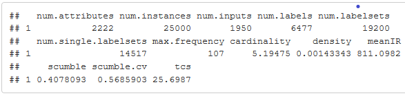
As we know the value of scumble lies in the range [0,1], and a low score would denote an MLD with not much concurrence among imbalanced labels and the resampling algorithms would work better. Here we can see a scumble value of 0.4078238, which is a high score, implying there is a good amount of concurrence among imbalanced labels, making it a difficult classification problem. IRLbl value(meanIR) is also quite high indicating a good amount of imbalance.
Labels’ information in the MLD, including the number of times they appear, their IRLbl and SCUMBLE measures, can be retrieved by using the labels member of the mldr class.
#inspect first 10 labels
head(eurlex$labels, 10)
## index count freq IRLbl
## abandoned_land_ 2313 4 1.666667e-04 632.25000
## abolition_of_customs_duties_ 2314 8 3.333333e-04 316.12500
## abruzzi_ 2315 1 4.166667e-05 2529.00000
## access_to_a_profession_ 2316 5 2.083333e-04 505.80000
## access_to_community_information_ 2317 26 1.083333e-03 97.26923
## access_to_education_ 2318 1 4.166667e-05 2529.00000
## access_to_information_ 2319 60 2.500000e-03 42.15000
## access_to_the_courts_ 2320 3 1.250000e-04 843.00000
## accession_criteria_ 2321 3 1.250000e-04 843.00000
## accession_negotiations_ 2322 3 1.250000e-04 843.00000
## SCUMBLE SCUMBLE.CV
## abandoned_land_ 0.7280804 0.049854037
## abolition_of_customs_duties_ 0.6987362 0.188424548
## abruzzi_ 0.9163142 NA
## access_to_a_profession_ 0.6149454 0.101608404
## access_to_community_information_ 0.3241009 0.560816073
## access_to_education_ 0.7741105 NA
## access_to_information_ 0.4354458 0.469904425
## access_to_the_courts_ 0.6962987 0.036354777
## accession_criteria_ 0.6720641 0.008151489
## accession_negotiations_ 0.6720641 0.008151489The mldr package provides a plot() function specific for dealing with “mldr” objects, allowing the generation of several specific types of plots. Otherwise the exploratory analysis of the MLD would have been tedious, as there are thousands of attributes and labels.
Concurrence (LC) Plot
The concurrence plot explores interactions among labels. This plot has a circular shape, with the circumference partitioned into many disjoint arcs representing labels. Each arc has length proportional to the number of instances where the label is present. These arcs are in turn divided into bands that join two of them, showing the relation between the corresponding labels. The width of each band is proportional to the number of instances in which both labels appear simultaneously. Since drawing interactions among all the labels can produce a confusing result, we have plotted for some labels containing terms - water, pollution and employment.
We can choose the labels from the mldr attribute eurlex$labels. But, the plots of mldr use eurlex$attributes, and they contain all features and labels. So we need to find those labels’ indices in eurlex$attributes. eurlex$attributes first start with features and then followed by labels.
head(eurlex$attributes)## abide ability able abolish abolition
## "numeric" "numeric" "numeric" "numeric" "numeric"
## abovementioned
## "numeric"tail(eurlex$attributes)## zambia_ zimbabwe_ zinc_ zoo_ zoology_ zoonosis_
## "{0,1}" "{0,1}" "{0,1}" "{0,1}" "{0,1}" "{0,1}"plot_labels <- grep('water|employment|pollution',rownames(eurlex[["labels"]])) + (eurlex$measures$num.attributes - eurlex$measures$num.labels)
head(names(eurlex$attributes)[plot_labels])## [1] "anti_pollution_device_" "atmospheric_pollution_"
## [3] "bathing_water_" "chemical_pollution_"
## [5] "coastal_pollution_" "community_employment_policy_"We can plot the concurrence plot using the plot() using type “LC”
plot(eurlex, type="LC", labelIndices=plot_labels, title="Concurrence plot")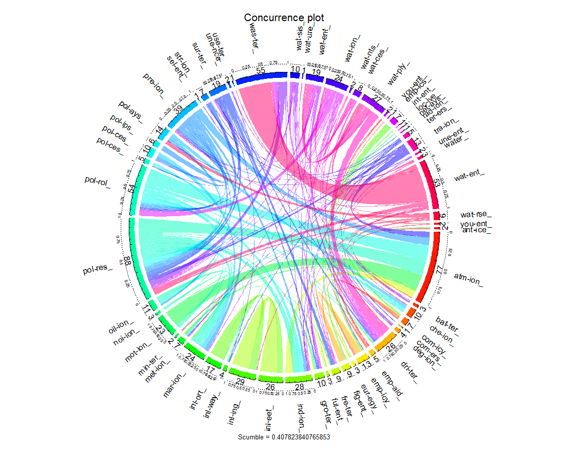
The names of the labels gets abbreviated in the plot. We can see from the fat pink band many instances are common to the categories/labels - water_treatment_ (wat_ent_) and wastewater_ (was_ter) as expected, and also we saw in top-k words/bigram that many words/bigrams were appearing common for these labels. Also bands emanating from pollution related labels pollution_control_ (pol_rol_) and pollution_control_measures_ (pol_res) meets the arc containing atmospheric_pollution_ (atm_ion), which implies many instances share labels atmosphere pollution and pollution control measures. We can also see the thin orange bands for labels - employment_policy_ (emp_icy) and fight_against_unemployment_ (fig_ent) sharing common instances, and they don’t meet the arcs containing pollution related instances, and even in top-k words/bigrams we had observed there were no common words between employment and pollution/water related labels. Also we see a lot of thread like bands appearing in the plot which implies many categories exist which have very less instances.
Label Histogram (LH) Plot
The label histogram relates labels and instances in a way that shows how well-represented labels are in general. The X axis is assigned to the number of instances and the Y axis to the amount of labels. In our plot the data is concentrated on the left side of the plot, which means that a great number of labels are appearing in very few instances.
plot(eurlex, type='LH',col = brewer.pal(11, 'Spectral'), title='Eurlex', xlim=c(0,10))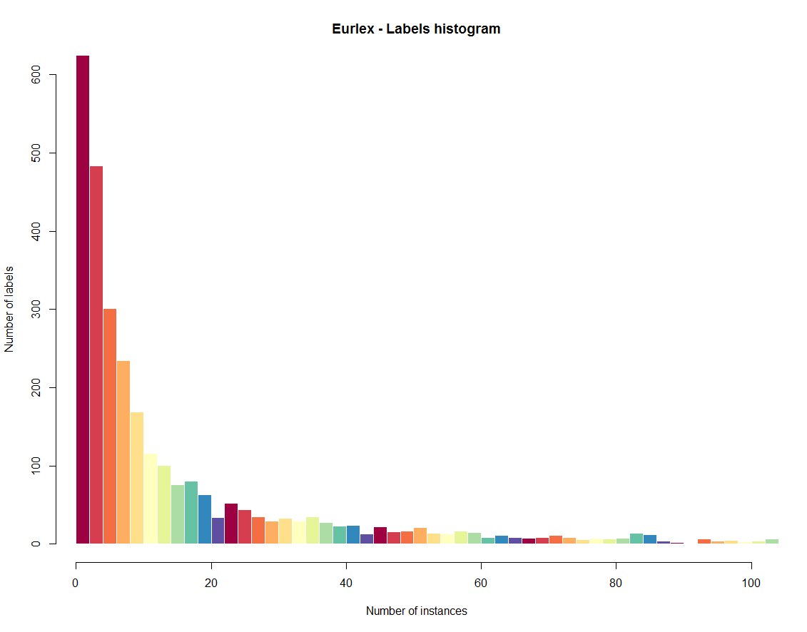
Labelset Histogram (LSH) Plot
The labelset histogram is similar to LH plot but, instead of representing the number of instances in which each label appears, it shows the amount of labelsets.
plot(eurlex, type='LSH',col = brewer.pal(11, 'Spectral'), title='Eurlex', xlim=c(1,10), ylim=c(0,2000))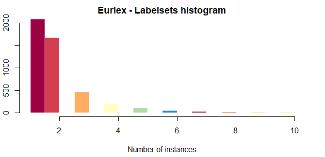
Label Bar (LB) Plot
The label bar plot display the number of instances for each one of the labels.
par(mar=c(10,2,2,2)+0.1)
plot(eurlex, type='LB',col = brewer.pal(11, 'Spectral'), title='Eurlex', labelIndices=plot_labels)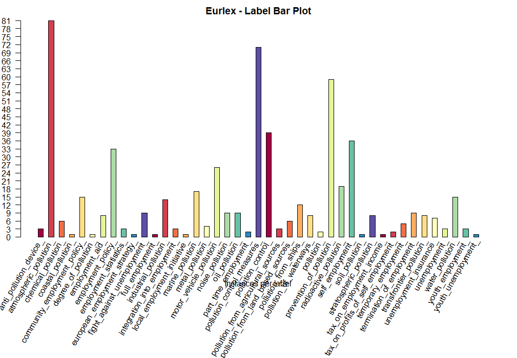
Cardinality Histogram (CH) Plot
The cardinality histogram represents the amount of labels instances have in general. Since data has accumulated on the left side of the plot it means that very less instances have a notable amount of labels.
plot(eurlex, type='CH',col = brewer.pal(11, 'Spectral'), title='Eurlex')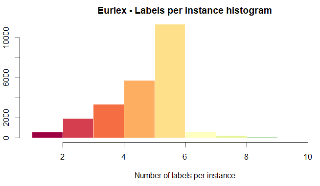
Tf-Idf and Term incidence as features
We come to the end of the exploratory analysis over the English text and the MLD dataset. From the above analysis it seems term-incidence and tf-idf can be surmised to be discriminatory features for the problem, as related labels/categories share many terms/bigrams. Also the concurrence plot helped us in observing related categories share many instances.